DITA Agent
An novel approach to object navigation in AI2-THOR. Code and resources, visualization are available here.
Abstract
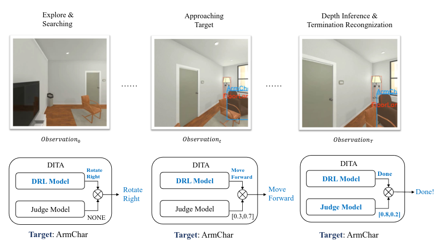
This project addresses the critical challenge of object navigation in autonomous navigation systems, particularly focusing on the problem of target approach and episode termination in environments with long optimal episode length in Deep Reinforcement Learning (DRL) based methods. While effective in environment exploration and object localization, conventional DRL methods often struggle with optimal path planning and termination recognition due to a lack of depth information.
To overcome these limitations, we propose a novel approach, namely the Depth-Inference Termination Agent (DITA), which incorporates a supervised model called Judge Model to implicitly infer object-wise depth and decide termination jointly with reinforcement learning. We train our judge model along with reinforcement learning in parallel and supervise the former efficiently by reward signal. Our evaluation shows the method is demonstrating superior performance, we achieve a 9.3% gain on success rate than our baseline method across all room types and gain 51.2% improvements on long episodes environment while maintaining slightly better SPL.
Method
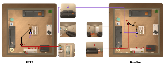
Despite the promising outcomes demonstrated by Deep Reinforcement Learning (DRL) based methods in the realms of exploration and object localization, their application in environments characterized by extended optimal episode lengths presents distinct challenges. They often struggle on addressing optimal path planning to the object, as well as termination recolonization. In these scenarios, our observations indicate that after the agent has seen the target object, it often still failed to keep approaching the target. These limitations become even more pronounced in object navigation, where the agents are expected to declare the termination of the episode on its own in unseen environments with the absence of depth information. Given that objects of varying types often exhibit different sizes, it becomes challenging for DRL agents to discern the dependencies between their actions and the task at hand without explicit depth information pertaining to the object, resulting in the navigation agent falling into local maximums, in which it avoids step penalty by terminating the episode in the early stage in environments.
Inspired by these observations, we present a novel approach for object navigation, utilizing DRL rewards to guide a model to implicitly infer depth. Our method introduces a model called the Judge Model, a supervised classification model trained alongside the DRL agent and guided by the DRL reward signal. The judge model determines the appropriate termination time with DRL by implicitly estimating object depth from object detection results. We integrate our judge model as part of the agent, enabling the DRL agent to explore the unseen environment while searching for the target. Once the target appears in the observation frame, the judge model provides a termination confidence level. The agent then decides whether to terminate the episode based on the outputs from both models. We evaluate our proposed DITA model in AI2-THOR framework, a platform that furnishes highly customizable environments, and permits the agent to enact navigation actions within these environments, subsequently observing the changes induced by those actions.
Object Navigation
Consider an environment set that has object types \(C = \{c_1,c_2,...,c_n\}\), the aim of object navigation is to navigate to a specified object type \(c_{target} \in C\), e.g., an “ArmChair” or “Pillow”. The agent is initially placed randomly at state \(t_0\), in each time step \(t\), it takes observation \(o_t\) and acts in the environment. \(o_t \in O\) is a visual input of RGB image from the camera of the agent, whereas the agent has the action space of six discrete actions \(a_t \in A =\)
\(\{MoveAhead, RotateLeft, RotateRight, LookUp, LookDown, Done\}\).
The action \(MoveAhead\) propels the agent forward \(0.25m\), rotational actions turn the agent \(45^\circ\) to the left or right and look actions adjust the camera by \(30^o\) upwards or downwards. The action \(Done\) enables the agent to declare success and terminate the episode. Termination conditions include the agent’s active termination or exceeding the maximum episode length. An episode is considered successful if the agent actively terminates with the target object within the observation frame and at a distance of less than \(1.5m\).
Deep Reinforcement Learning Branch
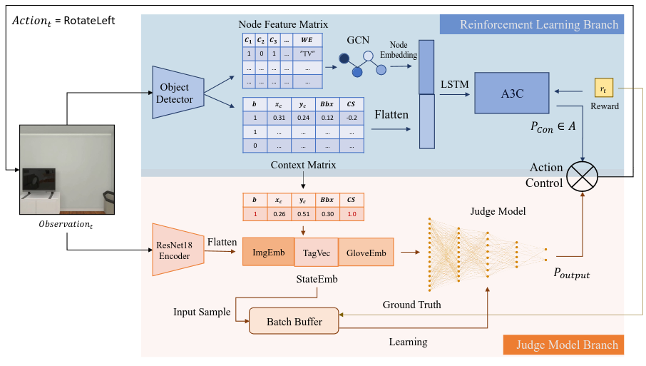
Given the impressive capabilities of enriched environment exploration ability of MJOLNIR-o, We use it as our backbone reinforcement learning model.
Upon receiving the observation, the model builds a 2-D array in shape \((N_C,N_C + 300)\) called Node Feature Matrix by processing the result from a ground-truth object detector, where \(N_C = mod(C)\) is the number of object types across all rooms. Each row of the Node Feature Matrix would be passed as an individual input node feature pass to the corresponding GCN node, with its first \(N_C\) columns standing for a binary vector indicating the object detection result for all object types \(C\), and the last 300 elements is a GloVe word embedding vector of the current object. Node embedding is learned through a graph neural network that was made by object relation labels provided by Visual Genome (VG) dataset and pruned some relations off for AI2-THOR objects.
On the other hand, the model also constructs Context Matrix from object detection, with each row representing a vector containing the object detection state of an object type \(c \in C\) with \(row_c = \{b,x_c,y_c,Bbx,CS\}\), b is a binary indicator represents whether an object with type \(c\) is visible in the current frame, \(x_c\) and \(y_c\) is the coordinates of object detection bounding box center, \(Bbx\) is the bounding box area, and the \(CS\) is the cosine similarity of word embedding vectors between object type \(c\) and the target object type, defined as:
\(CS(G_{c},G_{target}) = \frac{G_{c} \cdot G_{target}}{||G_{c}|| \cdot ||G_{target}||}\).
Our evaluation of the environment points out that sometimes more than one instance of object type \(c\) could be visible, deals with this by averaging their bounding box center and area by default, but if two instances with the identical object type of large size show in one frame, the averaged bounding box might cover a lot of irrelevant smaller objects with other types. Moreover, since our judge model will receive information from the context matrix as input, such an approach leads to the problem of providing dirty data. In contrast, when multiple instances of type \(c\) occur in the same frame, we take the one that with the largest \(Bbx\) to represent the class. The learned node embedding and the flattened context matrix are concatenated as joint embedding, passed to an LSTM cell, and send to the A3C model to learn the control action distribution \(P_{con}\).
Judge Model Branch
In each time step \(t\), if \(Done\) is sampled by the DRL branch, judge model branch processes the flattened image feature \(ImgEmb_t\) of the observation, extracted via a pre-trained ResNet-18 encoder. This encoder is pre-trained on ImageNet, encompassing 1000 object classes. By evaluating the context matrix obtained from the reinforcement learning branch, the judge model branch selects the target row with \(CS = 1.0\) as the target state vector. The image features \(ImgEmb_t\), target state vector \(TagVec_t\) from the context matrix, and glove word embedding of the target \(GloveEmb_t\) are concatenated to form a state embedding \(StateEmb_t\).
The judge model is trained only on Effective States — states where the target is visible in the observation. If the target is not visible in the current frame (as indicated by \(b=0\) in \(StateEmb_t\)), the current time step is ignored by the judge model, yielding no output. If the target is visible, \(StateEmb_t\) is passed to the judge model. The output is then forwarded to the action control module. The agent acts on the final output action decided by the action control model and receives the reward signal. Analysis of the reward range reveals that successful episodes yield rewards in the range \(R_t \in [4.05,4.90]\). If \(R_t >= 4.0\), the ground truth for time step \(t\) is set as positive; otherwise, it’s set as negative. The ground truth of time step \(t\) and the \(StateEmb\) are stored as learning data in a “Batch Buffer” with a capacity of 64 samples. Upon reaching the maximum batch size, these samples serve as a training batch for the judge model to update the weights.
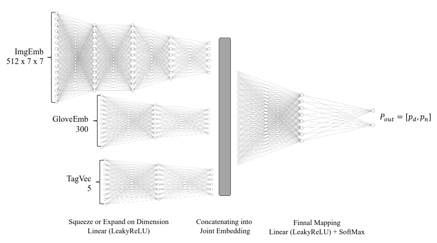
Judge model is a supervised binary classification neural network with expanding and squeezing layers, these layers map the input \(StateEmb\) into the same dimension by several stacked linear layers, since \(GloveEmb\) might contain negative floating numbers, we observe that applying ReLU activation after linear layers causes the gradient of large partition of neurons to be zero, therefore we use Leaky ReLU activation following the linear layers to prevent dead ReLU problem. Eventually, concatenate \(ImgEmb\), \(GloveEmb\), and \(TecVec\) together to form a joint embedding, output the classification result with probabilities for whether to sample termination.
In addition, because our data is collected online by reinforcement learning, during an episode, as mentioned in section, since the success condition requires the agent to terminate within a certain range of the target, most of the Effective States comes with ground truth of the negative class, where the agent should not terminate, this imbalance of training data causes long tail problem. In our method, we use Focal Loss as our loss function as an alternative to Cross Entropy Loss:
\[FL(p_t) = -(1-p_t)^\gamma log(p_t)\]Focal loss dynamically adjusts the weight of each instance in the loss function, focusing more on hard-to-classify instances and less on easy ones. We set \(\gamma = 0.7\) in our experiments.
Action Control
Action control directly samples the action from the output of reinforcement learning branch \(P_{con}\) in training. During testing, based on probability distribution from the outputs of two models \(P_{con}\) and \(P_{out}\), the action model outputs the final action \(a_t = Done\) if both models are confident enough to terminate the episode, specifically, note the probability output of action Done from \(P_{con}\) as \(p_{\lambda}\), and the probability of sample termination action in \(P_{out}\) as \(p_d\), output \(a_t = Done\) when the sum of the confidence for termination action in two distributions satisfies \(p_{d} + p_{\lambda} >= 1.5\).
Otherwise, according to the output of judge model, while \(p_{d}\) is sampled from the output of judge model, action control outputs final action \(a_t \in P_{con}\). Whereas if \(p_n\) is sampled, action control outputs final action \(a_t \in P_{sub}\) with \(P_{sub}\) being a subset of \(P_{con}\) without Done action. This is formally shown in equation.
Experiment Result
We use AI2-THOR as our environment simulator to evaluate our method for object navigation. AI2-THOR contains 120 different rooms with 30 rooms per room type Kitchen, Bedroom, Living room, and Bathroom. The rooms were split ass training data and testing data, in our experiments, we use 80 rooms as training data, with 20 rooms from each room type. The remaining 40 rooms were used for testing. Amount all object categories in AI2-THOR environment \(mod(C_{total})=101\).
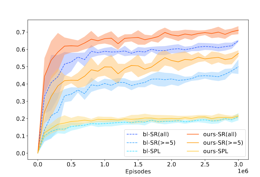
Models were compared based on two metrics. Success Rate (SR)measures the probability of agent success in the environment, computed by \(SR=\frac{1}{N} \sum_{n=0}^N S_n\), \(N\) is the number of total episodes in evaluation, and $S_n$ is a binary indicator with $S_n=1$ represents agent succeed in episode $n$. In addition, we use \textit{Success Weighted by Path Length (SPL)}, which measures the navigation efficiency of the agent, defined as \(SPL=\frac{1}{N} \sum_{n=0}^N S_n \frac{O_n}{max(L_n,O_n)}\) Where $O_n$ is the length of the optimal path to the target that agent could take in episode \(n\), \(L_n\) is the actual path length agent has taken.
| All | L >= 5 | ||||
|---|---|---|---|---|---|
| SR(%) | SPL(%) | SR(%) | SPL(%) | ||
| Random | 10.4 | 3.2 | 0.6 | 0.4 | |
| Target-driven VN | 35.0 | 10.3 | 25.0 | 10.5 | |
| Scene Prior | 35.4 | 10.9 | 23.8 | 10.7 | |
| SAVN | 35.7 | 9.3 | 23.9 | 9.4 | |
| MJOLNIR-r | 54.8 | 19.2 | 41.7 | 18.9 | |
| MJOLNIR-o | 65.3 | 21.1 | 50.0 | 20.9 | |
| DITA (Ours) | 71.4 | 21.6 | 57.9 | 22.2 | |
For detailed result please refer to the paper.