Recognizing Road Environments and Implementing Inner Road Markings for AGV Navigation: A Simulation-to-Reality Approach in NVIDIA Omniverse. Supervised by Professor Chun-Yi Lee, Department of Computer Science, National Tsing Hua University.
Overview
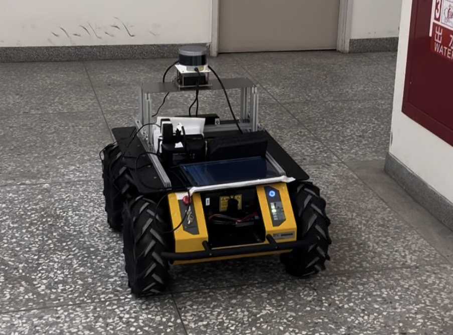
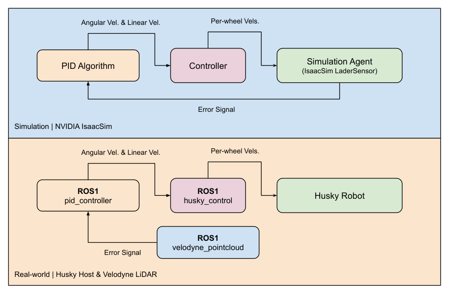
Painting lines on highways puts road workers next to live traffic. This industry-academia project automates the task with a Husky robot that follows the roadside wall at a fixed distance and draws a line as it drives. A Velodyne VLP-16 LiDAR measures the distance to the wall, and a Proportional-Integral-Derivative (PID) controller turns that distance error into velocity commands.
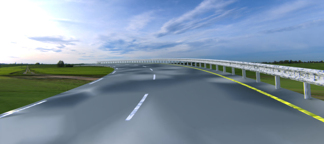
The controller was first developed and tuned in NVIDIA Isaac Sim, inside a custom highway scene with straight sections, left and right curves, and concrete and steel barriers. It was then deployed on the real robot through ROS1 to check that the simulated behaviour holds in the physical world.
Background
PID control
The controller computes the control signal \(u(t)\) from the error \(e(t)\) between a setpoint and the measured value:
\[u(t) = K_p e(t) + K_i \int_0^t e(\tau)\,d\tau + K_d \frac{de(t)}{dt}\]The proportional term corrects the current error, the integral term removes steady-state error, and the derivative term damps the response by reacting to the rate of change. Here the error is the difference between the current LiDAR reading \(L_s\) and the desired wall distance \(L_d\):
\[e(t) = L_s - L_d\]Hardware
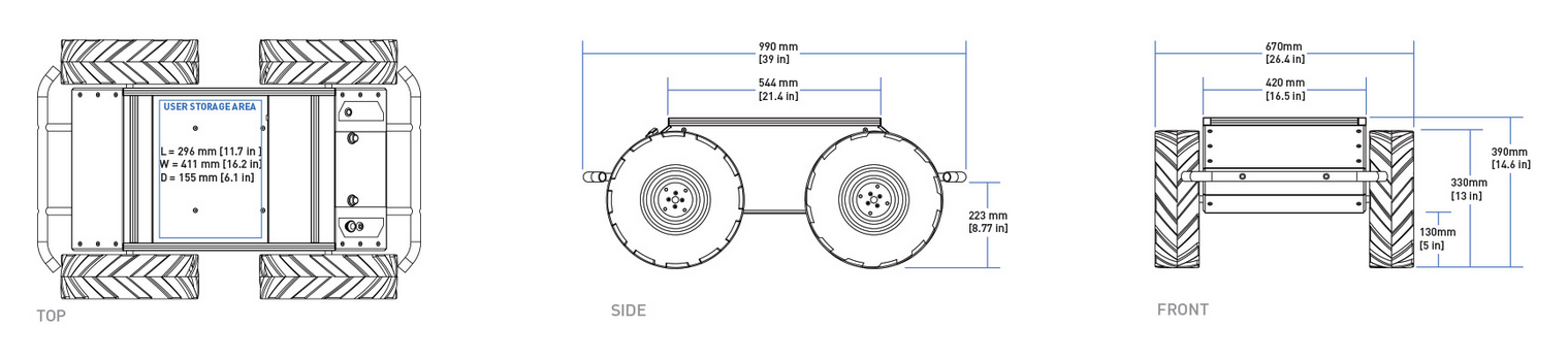
- Robot platform. The Clearpath Husky A200 is an all-terrain unmanned ground vehicle with a rugged chassis and a flexible payload area for sensors and compute.
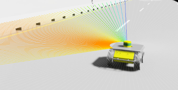
- LiDAR. The Velodyne VLP-16 is a 3D laser scanner that measures distance from the time of flight of its laser pulses. Its point cloud gives the robot its distance to the wall in real time.
Software
- Simulation. NVIDIA Isaac Sim 2022.2.1 provides physics-based robot models and sensor simulation, so the controller can be tested in a controlled and repeatable way before touching hardware.
- ROS1. The Robot Operating System connects the LiDAR driver, the PID controller and the Husky base controller through topics, so each part runs as its own node.
Simulation environment
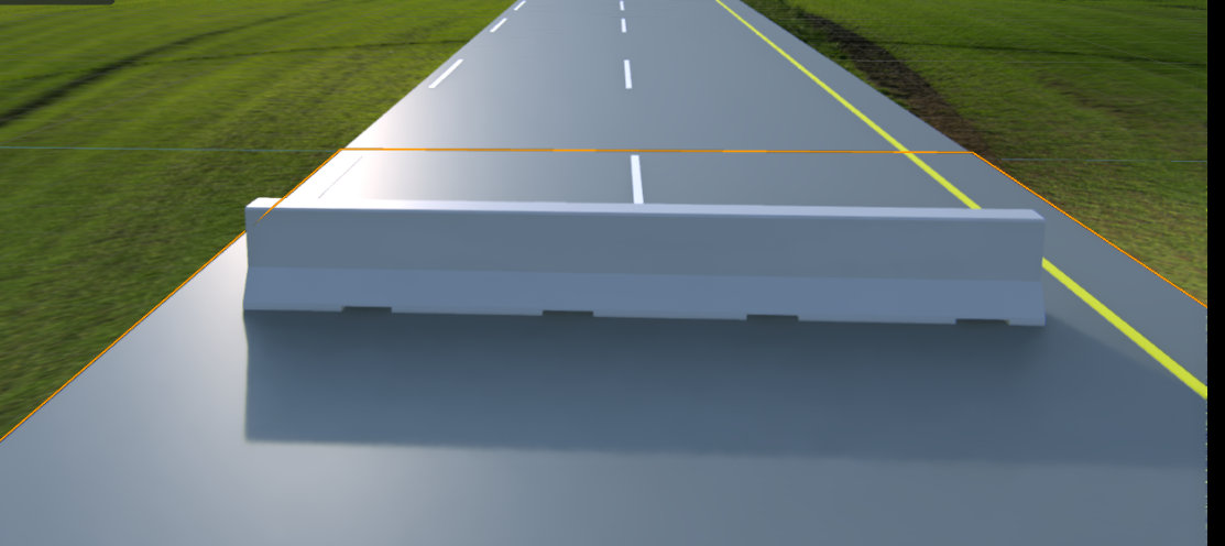
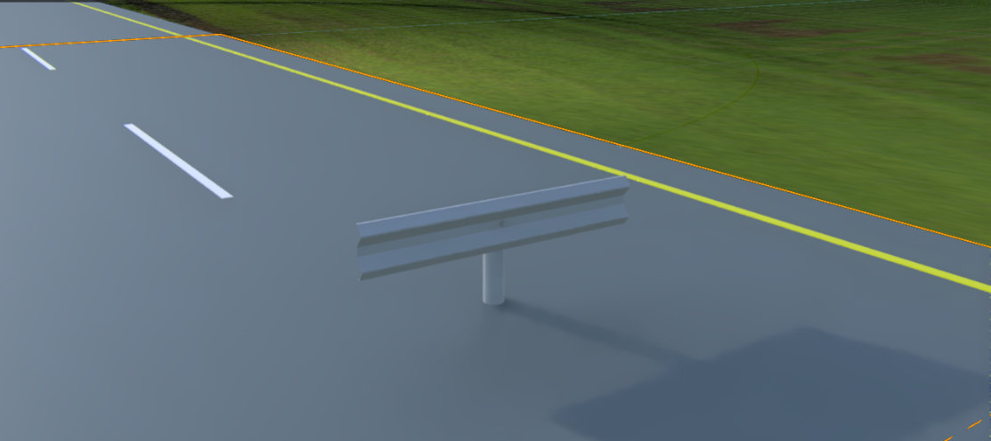
The highway assets, road pieces and barrier types, were modelled in Unity3D, exported as FBX and converted to USD so that Isaac Sim can load them. The scene, robot model and lighting are combined in one USD stage that main.py loads before running the controller. Isaac Sim was used through three workflows: the GUI to build the highway, extensions for the built-in LiDAR, and standalone Python to run the evaluation.
Method
LiDAR interpretation
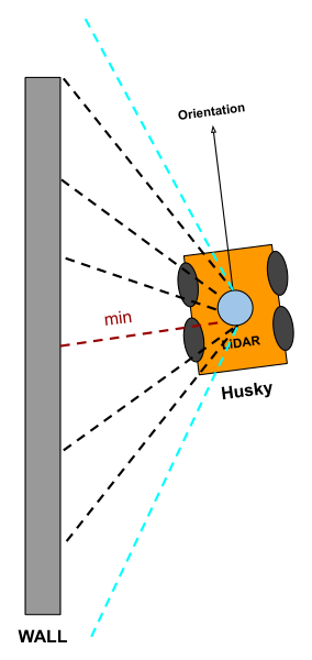
The full scan \(R_{lidar}\) is filtered to the side facing the wall, \(0^\circ\) to \(180^\circ\) for the left or \(180^\circ\) to \(360^\circ\) for the right. The shortest remaining reading is the robot’s estimated distance to the wall, and it is passed to the PID error as \(L_s\):
\[r_{min} = \min r_{lidar}, \quad r_{lidar} \in R_{lidar}\]The simulated LiDAR was configured to match the real VLP-16:
| Parameter | Value | Meaning |
|---|---|---|
| HrzFov | 20.0° | Horizontal field of view |
| HrzRes | 0.4° | Angle between rays on the horizontal axis |
| VrtFov | 30.0° | Vertical field of view |
| VrtRes | 2.0° | Angle between rays on the vertical axis |
| MaxRange | 100.0 m | Maximum detection range |
| MinRange | 0.4 m | Minimum detection range |
| RotationRate | 20.0 Hz | Sensor rotation rate |
Control
The PID step, Road_maker.adjust(), takes the current wall distance and returns an abstract velocity command made of an angular and a linear velocity:
A custom controller, a subclass of Isaac Sim’s BaseController, converts this command into per-wheel velocities for the skid-steer base, where \(\alpha\) is the wheel base and \(\beta\) the wheel radius:
Results
Simulation
In simulation the best gains were \(K_p, K_i, K_d = \{1.8, 0, 0\}\), so proportional control alone was enough. The simulated controller does not support turning in place, so the robot first drives forward without drawing until the PID loop settles, returns to the start, and then draws a smooth line. All three gains can be changed from the command line.
Real robot
On the real Husky the loop runs as three ROS1 nodes:
-
velodyne_pointcloudpublishes the LiDAR scan on/scan, with raw points on/velodyne_points. -
pid_controllersubscribes to/scan, runs the PID step and publishesgeometry_msgs/Twistcommands oncmd_vel. -
husky_controlsubscribes tocmd_veland turns the command into per-wheel velocities.
The real dynamics differ slightly from the simulated ones, and the best real-world gains were \(K_p, K_i, K_d = \{3.05, 0, 1.2\}\). The real base can turn in place, so it settles within a short distance and does not need the drive-and-return step used in simulation.
Lessons learned
- Dynamics mismatch. Simulated and real dynamics are never identical, so the gains need a short re-tuning pass on hardware.
- Speed sensitivity. Wall following was stable at linear speeds of 0.1 to 0.3 m/s on the real robot.
- Simulation first. Building the scene in Isaac Sim made testing faster, safer and repeatable. The project estimates the time saved compared with developing directly on the robot:
| Stage | Direct robot (weeks) | Simulation (weeks) | Time saved |
|---|---|---|---|
| Setup | 4–12 | 1–2 | 60%–90% |
| Testing and iteration | 6–18 | 4–10 | 50%–67% |
| Debugging | 2–6 | 1–2 | 50%–67% |
Future work
The current system needs a wall beside the road to follow. A vision-based path planner that follows the lane itself, combined with LiDAR for real-time obstacle avoidance, would remove that requirement.
Resources
- Simulation source code and documentation
- Real robot (ROS1) source code and documentation
- Simulation demonstration video
- Real-world demonstration videos
References
- M. Quigley. ROS: an open-source Robot Operating System. IEEE International Conference on Robotics and Automation, 2009.
- H. Suwoyo et al. Improving a Wall-Following Robot Performance with a PID-Genetic Algorithm Controller. EECSI, 2018. doi:10.1109/EECSI.2018.8752907
- Z. Zhou et al. Towards Building AI-CPS with NVIDIA Isaac Sim: An Industrial Benchmark and Case Study for Robotics Manipulation. arXiv:2308.00055, 2023.